Gaussian Process
In the most simple term, one can think of Gaussian Process, GP as being distributions over functions. It is a supervised Machine Learning technique and was developed, in the attempt, to solve regression problems (Wikipedia). The cool thing about Gaussian Process is that we don't need a "parametric model" to fit the data. It learns using the kernel trick. For an introduction to these techniques, I would recommend the nice review by Prof Zoubin Ghahramani on Probabilistic Machine Learning and Artificial Intelligence . Other nice books for GPs are Gaussian Processes for Machine Learning by Carl Edward Rasmussen and Christopher K. I. Williams and Machine Learning - A Probabilistic Perspective by Kevin Murphy. Before going into the actual explanation of what a GP is, it is important to have a brief background of how to find the marginals and conditionals of a Multivariate Nomal Distribution. See Chapter 4 from Kevin Murphy's book.
Marginals and Conditionals
Consider a 2D Gaussian Distribution whose parameters are given by
\begin{align} \boldsymbol{\mu}=\left(\begin{matrix} \mu_{1} \cr \mu_{2} \end{matrix}\right)\hspace{3cm}\boldsymbol{\Sigma}=\left(\begin{matrix} \Sigma_{11} & \Sigma_{12}\cr \Sigma_{21} & \Sigma_{22} \end{matrix}\right) \end{align}
Then, the joint distribution of $x_{1}$ and $x_{2}$, that is, $\mathcal{P}\left(x_{1},\,x_{2}\right)$ can be written as
\begin{align} \mathcal{P}\left(x_{1},\,x_{2}\right)=\dfrac{1}{\left|2\pi\boldsymbol{\Sigma}\right|^{\frac{1}{2}}}\,\textrm{exp}\left[-\dfrac{1}{2}\left(\mathbf{x}-\boldsymbol{\mu}\right)^{\textrm{T}}\boldsymbol{\Sigma}^{-1}\left(\mathbf{x}-\boldsymbol{\mu}\right)\right] \label{eq:2d_gaussian} \end{align}
Using $\mathcal{P}\left(x_{1},\,x_{2}\right)=\mathcal{P}\left(x_{1}\left|x_{2}\right.\right)\mathcal{P}\left(x_{2}\right)$, it can be shown that the conditional $\mathcal{P}\left(x_{1}\left|x_{2}\right.\right)$ is also a quadratic with the mean and variance given by
\begin{align} \mu_{1\left|2\right.}=\mu_{1}+\Sigma_{12}\Sigma_{22}^{-1}\left(x_{2}-\mu_{2}\right)\hspace{3cm}\Sigma_{1\left|2\right.}=\Sigma_{11}-\Sigma_{12}\Sigma_{22}^{-1}\Sigma_{21} \label{eq:marginals} \end{align}
such that
\begin{align} \mathcal{P}\left(x_{1}\left|x_{2}\right.\right)=\dfrac{1}{\sqrt{2\pi\Sigma_{1\left|2\right.}}}\,\textrm{exp}\left[-\dfrac{1}{2}\left(\dfrac{x_{1}-\mu_{1\left|2\right.}}{\Sigma_{1\left|2\right.}}\right)^{2}\right] \label{eq:marginals_distribution} \end{align}
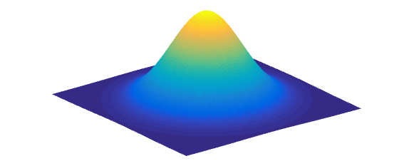
Intuitively, this can be understood by the fact that if we take a slice across a 2D Multivariate Normal Distribution as shown in the picture below, the resulting distribution is also a Gaussian Distribution.
GP for Regression
In Bayesian Parameter Inference, in which case we have a parametric model $\mathcal{M}$ and some data $\mathcal{D}$, we would want to infer the posterior distribution of the parameters, that is, $\mathcal{P}\left(\boldsymbol{\theta}\left|\mathcal{M},\,\mathcal{D}\right.\right)$. On the other hand, a GP in fact defines a prior over the functions itself, such that it can be mapped to a posterior given some data $\mathcal{D}$. In this section, we will show how we can take adavantage of the nice properties of the above to predict the likely value of a function for a given $x_{*}$. The major assumption we will make is that the testing set of data is from the same distribution as the training set of data.
Noise-Free Case
Suppose we have a set of data, $\mathcal{D}=\left\{ \left(x_{i},\,f_{i}\right)\right\}$ for $i=1,2,3,\ldots N$, where $f$ is assumed to be an observable without noise. Now, given $x_{*}$, we would like to predict $f_{*}$ as well as its variance, $\Sigma_{*}$. In a sense, we effectively want the posterior distributions of $f_{*}$ given $x_{*}$, $x$ and $f$. Using Bayes' Theorem, we can write
\begin{align} \mathcal{P}\left(\mathbf{f}\left|\mathbf{y},\,\mathbf{X}\right.\right)=\dfrac{\mathcal{P}\left(\mathbf{y}\left|\mathbf{X},\,\mathbf{f}\right.\right)\mathcal{P}\left(\mathbf{f}\left|\mathbf{X}\right.\right)}{\mathcal{P}\left(\mathbf{y}\left|\mathbf{X}\right.\right)} \label{eq:BayesTheorem} \end{align}
where $\mathcal{P}\left(\mathbf{f}\left|\mathbf{y},\,\mathbf{X}\right.\right)$ is the posterior distribution of the function, $\mathcal{P}\left(\mathbf{f}\left|\mathbf{X}\right.\right)$ is the prior, $\mathcal{P}\left(\mathbf{y}\left|\mathbf{X},\,\mathbf{f}\right.\right)$ is the likelihood and $\mathcal{P}\left(\mathbf{y}\left|\mathbf{X}\right.\right)$ is the marginal likelihood which is simply given by
\begin{align} \mathcal{P}\left(\mathbf{y}\left|\mathbf{X}\right.\right)=\int\mathcal{P}\left(\mathbf{y}\left|\mathbf{X},\,\mathbf{f}\right.\right)\mathcal{P}\left(\mathbf{f}\left|\mathbf{X}\right.\right)d\mathbf{f} \label{eq:marginal_likelihood} \end{align}
Given now a new data $x_{*}$, the posterior distribution of $f_{*}$ is simply obtained by marginalisation.
\begin{align} \mathcal{P}\left(y_{\ast}\left|\mathbf{y},\,\mathbf{X},\,x_{\ast}\right.\right)=\int\mathcal{P}\left(y_{\ast}\left|\mathbf{f},\,x_{\ast}\right.\right)\mathcal{P}\left(\mathbf{f}\left|\mathbf{y},\,\mathbf{X}\right.\right)\,d\mathbf{f} \end{align}
The prior on the regression function which is a Gaussian Process, GP denoted by
\begin{align} f\left(\mathbf{X}\right)\sim\textrm{GP}\left(\boldsymbol{\mu}\left(\mathbf{X}\right),\,\kappa\left(\mathbf{X},\,\mathbf{X}’\right)\right) \label{definition_gp} \end{align}
where $\boldsymbol{\mu}\left(\mathbf{X}\right)$ is the mean of the function while $\kappa\left(\mathbf{X},\,\mathbf{X}'\right)$ is the covariance matrix, which is constructed using a kernel. In particular, for this example, we will consider the squared-exponential kernel,
\begin{align} \kappa\left(x,\,x’\right)=\sigma^{2}\,\textrm{exp}\left(-\dfrac{\left(x-x’\right)^{2}}{2\ell^{2}}\right) \label{squared_exponential} \end{align}
where $\ell$ and $\sigma$ control the horizontal and vertical variations respectively. The kernel encapsulates the correlation between two datapoints. What we would ideally want is the following - if two datapoints are close to each other, that is, $x-x'\approx0$, we would expect strong correlation, while if $x-x'\rightarrow\infty$, there should be minumum correlation between $x$ and $x'$. The kernel trick allows us to easily implement this. Note that there exists various other kernel types (for more details refer to Gaussian Processes for Machine Learning by Carl Edward Rasmussen and Christopher K. I. Williams)
\begin{align} \kappa\left(x,\,x’\right)=\begin{cases} \begin{matrix} \sigma^{2}\cr 0 \end{matrix} & \begin{matrix} x-x’=0\cr x-x’\rightarrow\infty \end{matrix}\end{cases} \end{align}
For the regression problem, the joint distribution is given by $$ \left(\begin{matrix} \mathbf{f}\cr \mathbf{f}_{\ast} \end{matrix}\right)\sim\left(\left(\begin{matrix} \boldsymbol{\mu}\cr \boldsymbol{\mu}_{\ast} \end{matrix}\right),\,\left(\begin{matrix} \mathbf{K} & \mathbf{k}_{\ast}\cr \mathbf{k}_{\ast}^{\textrm{T}} & k_{\ast\ast} \end{matrix}\right)\right) $$
where $k_{**} = \kappa\left(\mathbf{X}_{*},\,\mathbf{X}_{*}\right)$. Using the above results given by Equations \eqref{eq:marginals}, the posterior distribution $\mathcal{P}\left(f_{*}\left|\mathbf{y},\,\mathbf{X},\,x_{*}\right.\right)$ is simply $$ \mathcal{P}\left(\mathbf{f}\left|\mathbf{X}_{*},\,\mathbf{X},\,\mathbf{f}\right.\right)=\mathcal{N}\left(\mathbf{f}_{*}\left|\boldsymbol{\mu}_{*},\,\boldsymbol{\Sigma}_{*}\right.\right) $$ where $$ \boldsymbol{\mu}_{*}=\boldsymbol{\mu}\left(\mathbf{X}_{*}\right)+\mathbf{k}_{*}^{\textrm{T}}\mathbf{K}^{-1}\left(\mathbf{f}-\boldsymbol{\mu}\left(\mathbf{X}\right)\right) $$ $$ \boldsymbol{\Sigma}_{*}=k_{**}-\mathbf{k}_{*}^{\textrm{T}}\mathbf{K}^{-1}\mathbf{k}_{*} $$ We would notionally assume a mean function equal to 0 and the kernel must be positive definite. Hence, $$ \boldsymbol{\mu}_{*}=\mathbf{k}_{*}^{\textrm{T}}\mathbf{K}^{-1}\mathbf{f} $$ $$ \boldsymbol{\Sigma}_{*}=k_{**}-\mathbf{k}_{*}^{\textrm{T}}\mathbf{K}^{-1}\mathbf{K}_{*} $$
Noisy Case
If instead, we were to observe a noisy function given by $y=f\left(x\right)+\epsilon$ where $\epsilon\sim\mathcal{N}\left(0,\,\sigma_n^2\right)$, the matrix $\mathbf{K}$ is simply given by $$ \mathbf{K}_n=\mathbf{K}+\sigma_n^2\mathbf{I} $$ assuming that the observed data is corrupted by the noise independently. Then the prediction for the new function along with its uncertainty is given by $$ \boldsymbol{\mu}_{*}=\mathbf{k}_{*}^{\textrm{T}}\mathbf{K}_{n}^{-1}\mathbf{f} $$ $$ \boldsymbol{\Sigma}_{*}=k_{**}-\mathbf{k}_{*}^{\textrm{T}}\mathbf{K}_{n}^{-1}\mathbf{k}_{*} $$Learning the Kernel Parameters
The way to estimate the parameters is via maxmising the marginal likelihood, $\mathcal{P}\left(\mathbf{y}\left|\mathbf{X}\right.\right)$ which is simply a multivariate Gaussian distribution given by $\mathcal{N}\left(\mathbf{y}\left|0,\,\mathbf{K}_{n}\right.\right)$. Hence, \begin{align} \textrm{log }\mathcal{P}\left(\mathbf{y}\left|\mathbf{X}\right.\right)=-\dfrac{1}{2}\left[\mathbf{y}^{\textrm{T}}\mathbf{K}_{n}^{-1}\mathbf{y}+\textrm{log}\left|\mathbf{K}_n \right|+N\textrm{log}\left(2\pi\right)\right] \end{align}
where $N$ is the number of test data points. Essentially, the third term is does not depend on the kernel parameters and is simply an additive constant. Hence, the derivative of the marginal likelihood $$ \dfrac{\partial}{\partial\theta_{j}}\textrm{log }\mathcal{P}\left(\mathbf{y}\left|\mathbf{X}\right.\right)=-\dfrac{1}{2}\left[\mathbf{y}^{\textrm{T}}\dfrac{\partial\mathbf{K}_{n}^{-1}}{\partial\theta_{j}}\mathbf{y}+\dfrac{\partial}{\partial\theta_{j}}\textrm{log}\left|\mathbf{K}_{n}\right|\right] $$
can further be simplified using the fact that $\dfrac{\partial\mathbf{K}_{n}^{-1}}{\partial\theta_{j}}=-\mathbf{K}_{n}^{-1}\dfrac{\partial\mathbf{K}_{n}}{\partial\theta_{j}}\mathbf{K}_{n}^{-1}$ and that $ \dfrac{\partial}{\partial\theta_{j}}\textrm{log}\left|\mathbf{K}_{n}\right|=\textrm{tr}\left(\mathbf{K}_{n}^{-1}\dfrac{\partial\mathbf{K}_{n}}{\partial\theta_{j}}\right)$ such that $$ \dfrac{\partial}{\partial\theta_{j}}\textrm{log }\mathcal{P}\left(\mathbf{y}\left|\mathbf{X}\right.\right)=\dfrac{1}{2}\left[\mathbf{y}^{\textrm{T}}\mathbf{K}_{n}^{-1}\dfrac{\partial\mathbf{K}_{n}}{\partial\theta_{j}}\mathbf{K}_{n}^{-1}\mathbf{y}-\textrm{tr}\left(\mathbf{K}_{n}^{-1}\dfrac{\partial\mathbf{K}_{n}}{\partial\theta_{j}}\right)\right] $$
Given that we now have the gradient, one could easily use an optimisation algorithm to estimate the hyper-parameters. An alternative method is to have a full Bayesian formalism for inferring the posterior distributions of the hyper-parameters.
Examples
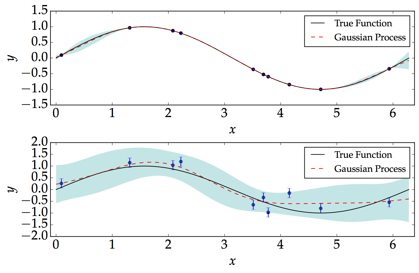
Below, we consider two examples: noise-free and a noisy. For the following, for illustration, we assume that the kernel parameters $\sigma$ and $\ell$ are both equal to 1. We show how the Gaussian Process performs well in the noise-free and equally-spaced data as shown below. We consider a simple sinusoidal function of the form $$ f=\textrm{sin}\left(x\right)\hspace{2cm}\left[0,\,2\pi\right] $$
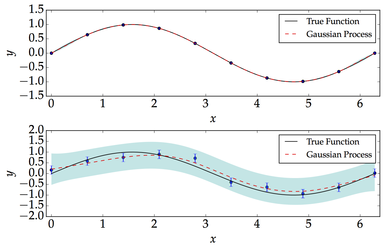
On the other hand, we generate noisy data, which are not equally-spaced. The point which we are mostly interested in is that the Gaussian Process basically demonstrates the level of confidence when we have or do not have data. As expected, we would be more confident when we have more data, and less confident when we don't have data.