An Introduction to Gibbs Sampling

Gibbs sampling is a variant of Markov Chain Monte Carlo (MCMC) method (Wikipedia). The idea is to update one of the parameters at a time, thus requiring conditional distributions. As with the standard Metropolis-Hastings algorithm, samples generated from an accumulated Gibbs chain are correlated with nearby samples and hence, if independent samples are required, it is desired to thin the chain by taking every n^th value. Moreover, the initial samples (burn-in) are negelected as they may not actually represent the underlying "true" distribution. The algorithm for Gibbs sampling is as follows:

1. Initialise $\boldsymbol{\theta}=\left(\theta_{0},\,\theta_{1},\,\ldots\theta_{n}\right)$.
2. Sample for the parameters as below:
• Sample $\theta_{0}'$ from $\theta_{0}\left|\theta_{0},\,\theta_{1},\,\ldots\theta_{n}\right.$.
• Sample $\theta_{1}'$ from $\theta_{1}\left|\theta_{0}',\,\theta_{2},\ldots\theta_{n}\right.$.
• $\vdots$
• Sample $\theta_{k}'$ from $\theta_{k}\left|\theta_{0}',\,\theta_{1}',\ldots,\,\theta_{k-1}',\,\theta_{k+1},\,\ldots\theta_{n}\right.$

However, notice that we need the conditional distributions. The advantage of Gibbs sampling is that it reduces the need for "tuning" as in the case for the Metropolis-Hastings algorithm. In particular, the starting point can be guessed or can be found using an optimisation algorithm.

Example - Bayesian Linear Regression

We consider a simple Bayesian Linear Regression to illustrate Gibbs sampling in practice. Suppose we have the datapoints, $\mathcal{D}=\left\{ x_{i},\,y_{i}\right\} $ for $i=1,\,2,\ldots N$ which have been generated from the model $y=\theta_{0}+\theta_{1}x$. In other words,

where $\epsilon\sim\mathcal{N}\left(0.0,\,\sigma_{n}^{2}\right)$. Our aim is the find the full posterior distributions of the parameters $\theta_{0}$ and $\theta_{1}$. The joint posterior distribution is simply

where we assume factorisable priors, that is, $\mathcal{P}\left(\theta_{0},\,\theta_{1}\right)=\mathcal{P}\left(\theta_{0}\right)\,\mathcal{P}\left(\theta_{1}\right)$ and we consider Gaussian priors such that,

Procedures

We first define the design matrices, $\mathbf{D}_{0}$, $\mathbf{D}_{1}$ and the vector $\mathbf{b}$ as follows:

As we assume $\sigma_{n}$ to be known, the likelihood can be written as

and the prior as

The dependence of $\theta_{0}$ in the log-joint posterior distribution, that is, $\theta_{0}\left|\theta_{1},\,\mathcal{D}\right.$ is simply

This is simply a quadratic function of $\theta_{0}$. If $a=\mathbf{D}_{0}^{\textrm{T}}\mathbf{D}_{0}+\dfrac{1}{\Sigma_{0}^{2}}$ and $b=2\theta_{1}\mathbf{D}_{0}^{\textrm{T}}\mathbf{D}_{1}-2\mathbf{b}^{\textrm{T}}\mathbf{D}_{0}-\dfrac{2\mu_{0}}{\Sigma_{0}^{2}}$, then

After completing the square,

This is a Gaussian distribution with mean, $\mu$ and standard deviation, $\sigma$ given by

Similarly, it can be shown that the dependence of $\theta_{1}$ in the joint posterior distribution, that is, $\mathcal{P}\left(\theta_{1}\left|\theta_{0},\,\mathcal{D}\right.\right)$ is Gaussian with

Python Code

Now we have all the mathematical tools to write the Python code. The simulated data is available on Github. We first define the linear function and the true parameters (for the gradient, $\theta_{1}$ and the y-intercept, $\theta_{0}$) are 2.0 and 0.5. Note that in the code below, we have used m and c for the gradient and the y-intercept. We also the specify the fraction of the chain that we will later consider as burn-in.

def linear(params):
	return params[0]*x + params[1]

# True Parameters
grad  = 2.0
yint  = 0.5

# Fraction considered as burn-in
frac  = 0.2

# Load the data 
data  = np.loadtxt('data_gibbs.txt')
x     = data[:,0]; xmin = min(x); xmax = max(x)
y     = data[:,1]
sigma = data[:,2]

The next step is to create the design matrices $\mathbf{D}_{0}$, $\mathbf{D}_{1}$ and the vector $\mathbf{b}$. We also define the hyper-parameters for the Gaussian priors, followed by defining functions to sample for $m$ and $c$ respectively. We add another function which we will then use to optimize the best-fit parameters. These parameters are then used as the starting point in the Gibbs Sampling scheme.

# Create Design Matrices
Dm = x/sigma
Dc = 1.0/sigma
b  = y/sigma

# Define Priors (Gaussian Priors)
mu_m = 2.0; mu_c = 1.0
si_m = 2.0; si_c = 2.0

# Define Functions for Sampling
def sample_grad(m, c):
	var  = 1.0/(np.dot(Dm.T, Dm) + 1.0/si_m**2)
	mean = var*(np.dot(b.T, Dm) + (mu_m/si_m**2) - c * np.dot(Dc.T, Dm))
	return np.random.normal(mean, np.sqrt(var))

def sample_yint(m, c):
	var  = 1.0/(np.dot(Dc.T, Dc) + 1.0/si_c**2)
	mean = var*(np.dot(b.T, Dc) + (mu_c/si_c**2) - m * np.dot(Dc.T, Dm))	
	return np.random.normal(mean, np.sqrt(var))

# Define the log-likelihood for optimisation
def loglikelihood(theta, data, Sigma):
  theta0, theta1 = theta 
  model     = linear(theta)
  chiSquare = LA.norm((model - data)/Sigma)**2
  loglike   = -0.5 * (chiSquare) 
  return loglike

# Use, for example, Powell method for optimisation
chi_square = lambda *args: -2*loglikelihood(*args)
result     = op.minimize(chi_square, [1.0, 1.0], args=(y, sigma), method = 'Powell', tol = 1E-5)
theta_op   = np.array(result["x"])

m = theta_op[0]
c = theta_op[1]

We are now ready to run the sampler. In particular, we fix the number of iterations to 200 000 and we reject the first 20 % of the chains.

iters = 2E5
trace = np.zeros(shape = (int(iters), 2))

def gibbs(m, c):

	for i in range(int(iters)):
		m = sample_grad(m, c)
		c = sample_yint(m, c)
		trace[i,:] = np.array([m, c])

	return trace

samples = gibbs(m,c)
samples = samples[int(frac*iters):] # Reject first 20 % of the chains

We finally get our nice 2D posterior distribution of the parameters.

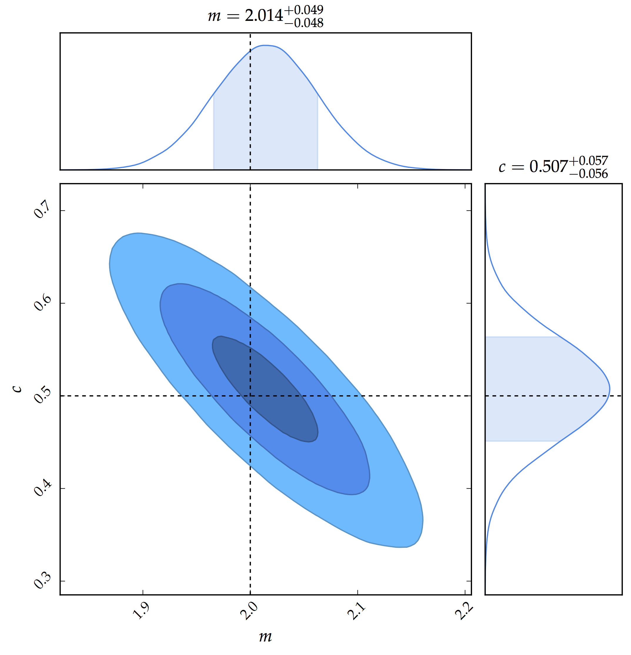
2D posterior plot of the two parameters