Sampling From Any Distribution
One of the recent topics which I had to study was how to sample from any distribution. While this seems to be a trivial question, Google did not help me much, although I did also try to post the problem on stackoverflow! Here, we will show three methods which we can use to generate random numbers from a distribution. In particular, we will look at some in-built functions in scipy, acceptance-rejection sampling and will consider interpolation method as well. The distribution which we will use is given by
\begin{align} \mathcal{P}\left(x\right) = \dfrac{k\,x^3}{e^{2x} - 0.1} \end{align}
where $k$ is the normalisation constant. Note that we will use the following notations: $\mathcal{P}\left(\centerdot\right)$ is the probability distribution function (PDF) while $\Phi\left(\centerdot\right)$ is the cumulative distribution function (CDF). The generic shape of this distribution follows that of a black body spectrum. This distribution is used only to illustrate the idea of sampling and we do not provide any relevant explanation to the actual physics of black body radiation in this post.
Using Scipy
The class rv_continuous in scipy.stats is straightforward to use. We simply need to define either the PDF or CDF using _pdf and _cdf respectively as shown below. We first define the PDF, followed by a function to normalise it. Note also that the PDF that we define in the class should be normalised.
x = np.linspace(0.0, 10.0, 1E4)

def p(x):
	return (x**3)/(np.exp(2.0 * x) - 0.1)

# Define function to normalise the PDF
def normalisation(x):
	return simps(p(x), x)

# Define the distribution using rv_continuous
class blackbody(ss.rv_continuous):
    def _pdf(self, x, const):
        return (1.0/const) * p(x)
We are now ready to use our above written functions to find $\mathcal{P}\left(x\right)$, $\Phi\left(x\right)$ and generate samples from the underlying distribution. We first need to instantiate it with the lower and upper limits given by a and b respectively. In principle, if not defined, it will be considered to be from $-\infty$ to $+\infty$.
blackbody_distribution = blackbody(name="blackbody_distribution", a=0.0)

# Find the normalisation constant first
norm_constant = normalisation(x)

# create pdf, cdf, random samples
pdf = blackbody_distribution.pdf(x = x, const = norm_constant)
cdf = blackbody_distribution.cdf(x = x, const = norm_constant)
samples = blackbody_distribution.rvs(const = norm_constant, size = 1E4)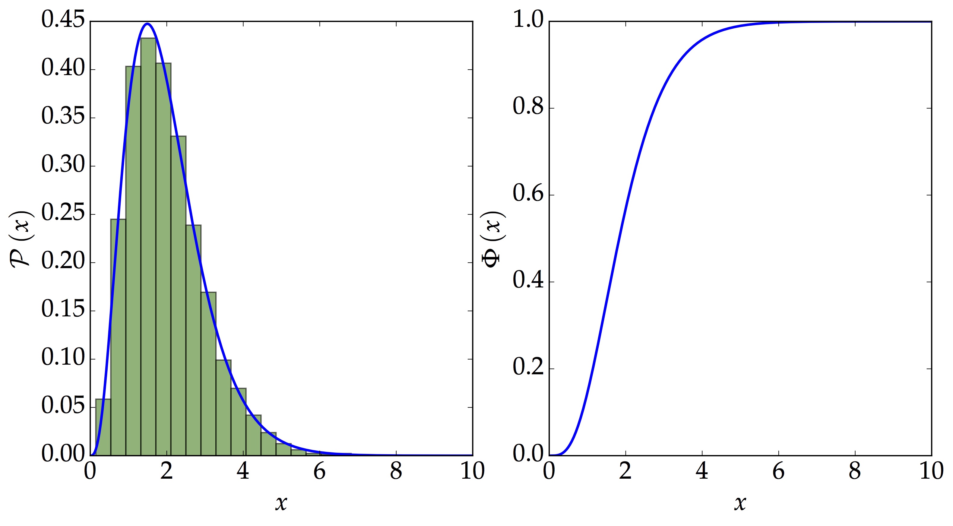
- Samples generated using
rv_continuousfromscipy.stats
The above plot shows the PDF, CDF and the samples generated from the distribution. In particular, we choose to draw 10 000 random samples. rv_continuous becomes useful when one needs more than just the samples. Once we have defined it, we can simply find other properties such as its mean, standard deviation and several more (see the documentation for further details).
Acceptance-Rejection Sampling
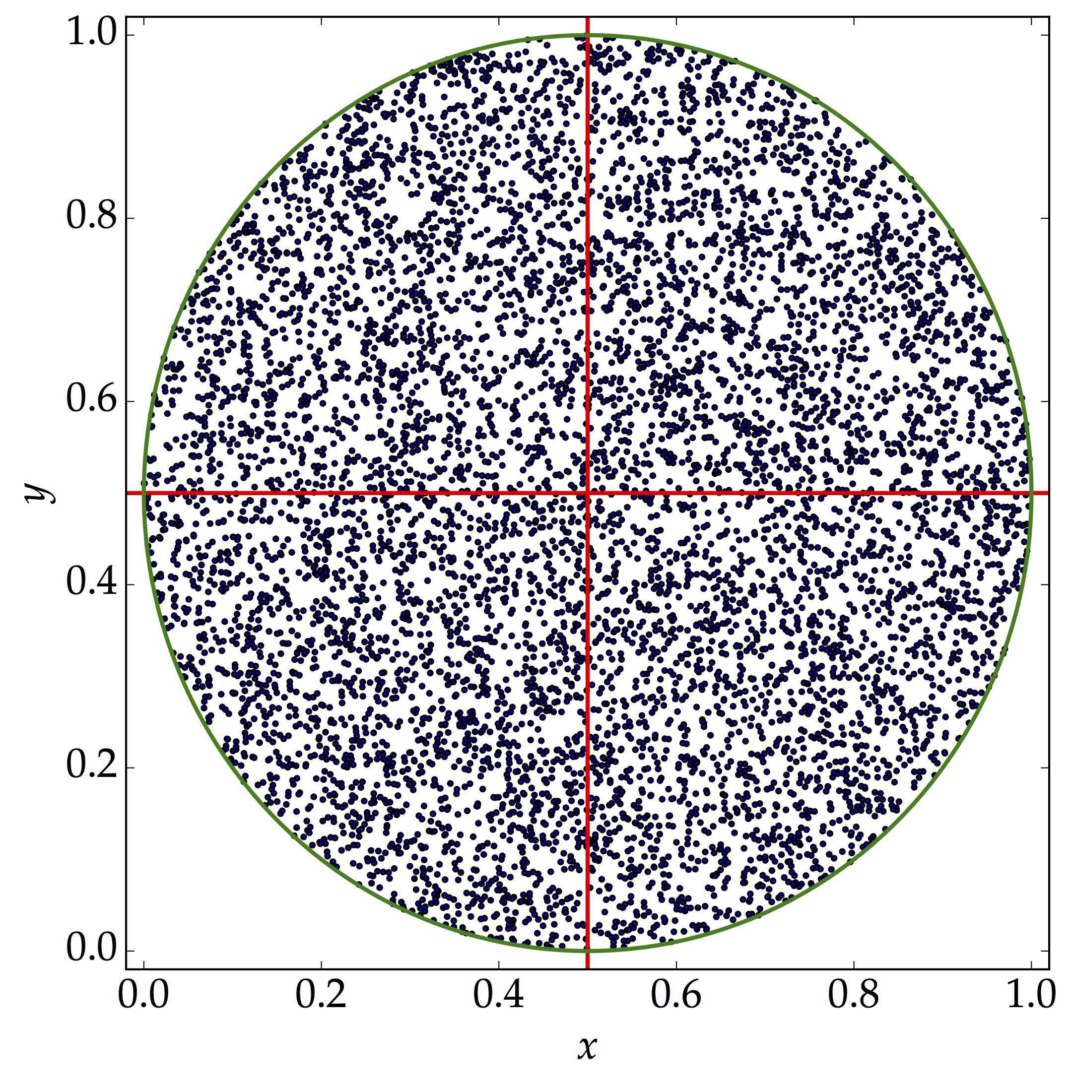
- Estimating value of $\pi$ using Monte Carlo Method
Imagine we have a square board of size $l$, on which there is a circle of radius $0.5l$ at the centre of the board, that is, at $\left(0.5l,0.5l\right)$ in a Cartesian coordinate system. We are throwing darts randomly on the board, say $N$ times. If $n$ is the number of times that the darts lie within the circle, the probability of throwing the darts successfully into the circle is simply $\frac{n}{N}$. This is also roughly equal to the ratio of the area of the circle to the area of the square board. One could use this idea to have a rough estimate of the value of $\pi$, that is,
\begin{align} \pi \approx 4 \times \frac{n}{N} \end{align}
As $N$ becomes larger, one would have a more accurate estimate of the number $\pi$. This is the idea behind Monte Carlo sampling. Through this lens, an alternative way to sample from a normalised distribution is to use acceptance-rejection sampling scheme. It is also sometimes referred to as Lahiri's Sampling method. This method is advantageous in the sense that we do not need to know the CDF. However, one downfall is that samples may get rejected very often. Moreover, say we want $N$ random numbers, it is unlikely that we will get that number of samples relatively easily. In this post, we have not implemented this method. In short,
suppose $X$ is a scalar random variable taking values in the interval $\left[a, b\right]$ according to the continuous probability density function $f\left(x\right)$. Let $M$ be an upper bound for $f$ on $\left[a, b\right]$, $M$ assumed finite. Choose $x$ uniformly in $\left[a, b\right]$. Then choose $u$ uniformly in $\left[0, M\right]$. If $u\leq f\left(x\right)$, we select $x$. Otherwise we reject $x$ and start over.
Interpolation Method
What do we do if neither of the two methods work but we do have the PDF? The procedures we adopt here is as follows:
- Find the CDF using
np.cumsum - Generate a random number from a uniform distribution, $\mathcal{U}\left[0,1\right]$
- Use
interp1dfromscipy.interpolateto estimate the random number.
# Our Own pdf, cdf and samples
own_pdf = p(x)/norm_constant
own_cdf = np.cumsum(own_pdf); own_cdf /= max(own_cdf)

# Define a function to return N samples
def genSamples(N):
	u = np.random.uniform(0, 1, int(N))
	func_interp = interp1d(own_cdf, x)
	samples = func_interp(u)
	return samples

own_samples = genSamples(1E4)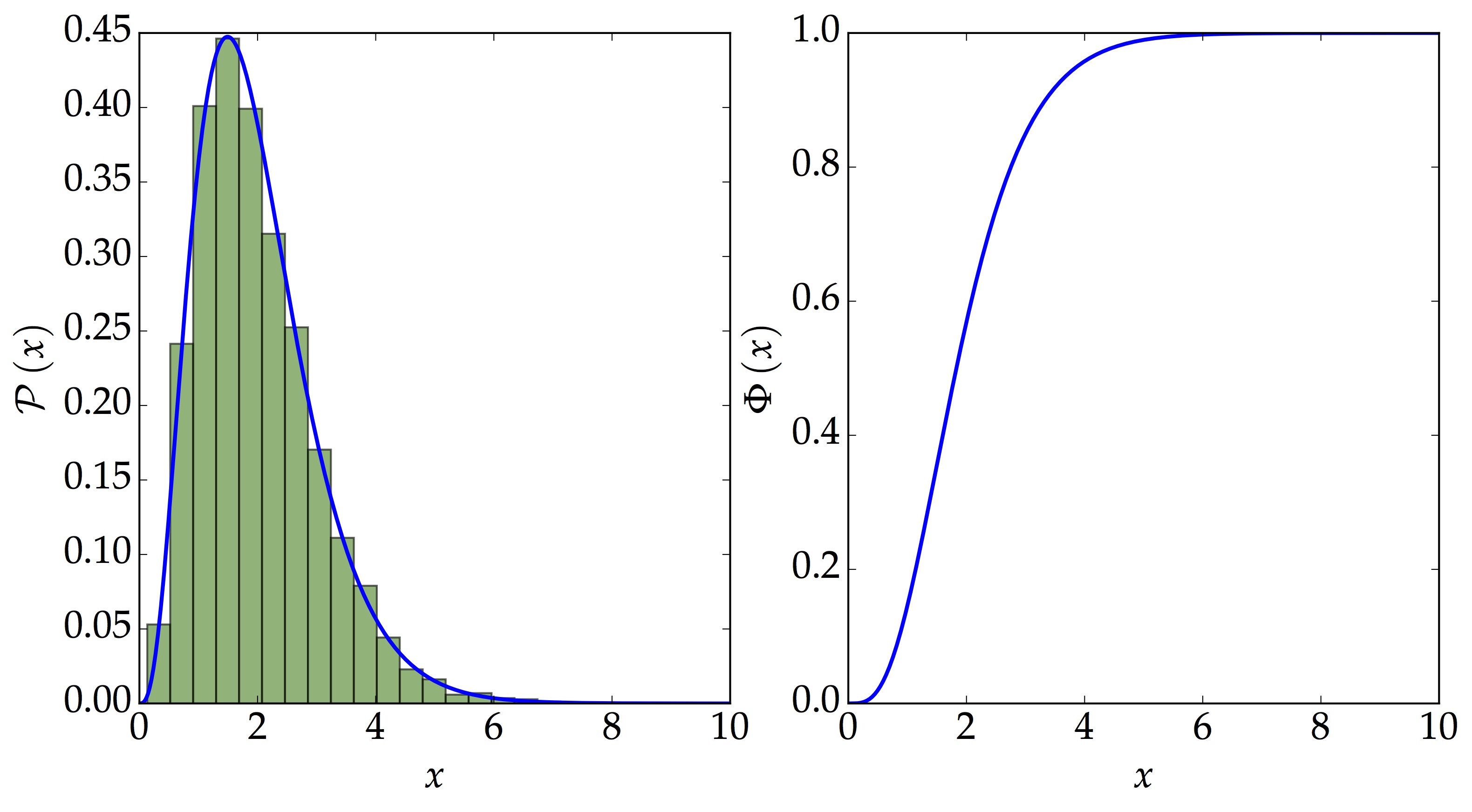
- Samples generated using the CDF and interpolation method
Here we have a nice distribution with 10 000 random samples drawn using the CDF. It looks similar to the one using rv_continuous!