Bayesian School 2016
The 2016 Bayesian School was organised at the University of Stellenbosch from the 21st to 25th November. In particular, the school focused on three main topics namely, Introductory Bayesian Methods, Monte Carlo Methods and Advanced Bayesian Methods which was taught by Prof. Alan Heavens from Imperial College.
Apart from the lectures, another interesting part of the school was "Research Hacks". The latter allows participants to meet in small groups, ask questions, exchange ideas and initiate collaboration. While these hacks predominantly followed the said-intentions, this also led to the publication of three papers (see arXiv:1704.03472, arXiv:1704.03467 and arXiv:1704.07830).
I learned quite a lot from Prof. Alan lectures and have also attempted some of the questions he proposed during the school. Also, there were various other interesting lectures, related to Bayesian methods. In particular, I will discuss two topics, namely KL Divergence and Bayesian Hierarchical Modelling below.
Kullback-Leibler (KL) Divergence
Suppose, we have a prior distribution which we denote as $\pi\left(\boldsymbol{\theta}\right)$ on the set of parameters $\boldsymbol{\theta}$. Afterwards, this is updated via Bayes' Theorem to a posterior distribution which we call $q\left(\boldsymbol{\theta}\right)$ and we want to know how much information we have gained from this update. This information can be quantified using the Kullback-Leibler (KL) Divergence, \begin{align} \textrm{D}_{\textrm{KL}}\left(q\left\Vert \pi\right.\right)=\int q\,\textrm{log}\left(\dfrac{q}{\pi}\right)d\theta \end{align} It is also referred to as the relative entropy. If this quantity is measured in base of logarithm of 2, the information gain is in bits, otherwise if measured in base of logarithm of $e$, the information gain is in nats. To illustrate the KL Divergence, let us consider a simple example, the KL Divergence of two Gaussians. Consider the prior and posterior distributions with means $\mu_{1},\,\mu_{2}$ and variances $\sigma_{1}^{2},\,\sigma_{2}^{2}$. The KL Divergence of $q$ from $\pi$ is $$ \textrm{D}\left(q\left\Vert \pi\right.\right)=\dfrac{\left(\mu_{1}-\mu_{2}\right)^{2}}{2\sigma_{1}^{2}}+\dfrac{\sigma_{2}^{2}}{2\sigma_{1}^{2}}-\dfrac{1}{2}-\textrm{log}\left(\dfrac{\sigma_{2}}{\sigma_{1}}\right) $$ From the above result, if the variance of the posterior distribution, that is, $\sigma_{2}^{2}$ decreases, then the information content increases, while if there is a huge difference between the two means, the information gain may increase significantly.
Another question related to KL Divergence was,
We have an experiment where a single datum $x$ is assumed to be drawn from a Gaussian Likelihood of mean $\mu$ and variance $\sigma^{2}$. Compute the KL divergence between an assumed Gaussian prior on $\mu$ (with mean zero and variance $\Sigma$) and the posterior.
For this question, the KL Divergence is given by $$ \textrm{D}_{\textrm{KL}}\left(q\left\Vert \pi\right.\right)=-\dfrac{1}{2}+\dfrac{\sigma^{2}}{2\left(\Sigma+\sigma^{2}\right)}+\dfrac{x^{2}\Sigma}{2\left(\Sigma+\sigma^{2}\right)^{2}}-\dfrac{1}{2}\textrm{log}\left(\dfrac{\sigma^{2}}{\Sigma+\sigma^{2}}\right) $$
If we had naively assumed a Dirac-Delta prior on the parameter, that is, $\Sigma=0$, then, $\textrm{D}_{\textrm{KL}}\left(q\left\Vert \pi\right.\right)=0$, which means there is no information gain. From my viewpoint, this example of computing the KL Divergence indicates the essence of incorporating priors in our analysis, which in turn leads us to advocating the Bayesian formalism.
Bayesian Hierarchical Modelling
This is also one of the topics which helped me to answer one of my questions: how do we proceed with parameter inference when we have error bars on both dependent and independent variables? The idea behind Bayesian Hierarchical Modelling (BHM) is to split the problem into steps where the full model now consists of a series of sub-models.
BHM links each sub-models, thereby propagating uncertainties from one sub-model to another. Let us consider a simple example, where we are fitting a straight line, $y=mx$ to a single data point, $X$ and $Y$. The complication is that both $X$ and $Y$ have errors, $\sigma_{X}$ and $\sigma_{Y}$ respectively. The question is: how do we infer $m$? In other words, we want $\mathcal{P}\left(m\left|X,\,Y\right.\right)$.
In this part, we will go through the steps in the BHM. To start with, we first need to write Bayes' Theorem, that is,
$$ \mathcal{P}\left(m\left|X,\,Y\right.\right)=\dfrac{\mathcal{P}\left(X,\,Y\left|m\right.\right)\mathcal{P}\left(m\right)}{\mathcal{P}\left(X,\,Y\right)}\propto\mathcal{P}\left(X,\,Y\left|m\right.\right)\mathcal{P}\left(m\right) $$We then introduce the so-called latent variables, $x$ and $y$ and since we are not interested in them, we will marginalise over them as follows,
$$ \mathcal{P}\left(m\left|X,\,Y\right.\right)\propto \int {\color{red}\mathcal{P}\left(X,\,Y,\,x,\,y\left|m\right.\right)}\mathcal{P}\left(m\right)dxdy $$Using the product rule, we have
$$ \mathcal{P}\left(m\left|X,\,Y\right.\right)\propto\int{\color{red}\mathcal{P}\left(X,\,Y\left|x,\,y,\,m\right.\right){\color{blue}\mathcal{P}\left(x,\,y\left|m\right.\right)}}\mathcal{P}\left(m\right)dxdy $$In this case, the first probability does not depend on $m$, that is, $\mathcal{P}\left(X,\,Y\left|x,\,y,\,m\right.\right) = \mathcal{P}\left(X,\,Y\left|x,\,y\right.\right)$ and using the product rule again, we have
$$ \mathcal{P}\left(m\left|X,\,Y\right.\right)\propto\int{\color{red}\mathcal{P}\left(X,\,Y\left|x,\,y\right.\right){\color{blue}{\color{magenta}\mathcal{P}\left(y\left|m,\,x\right.\right)}\mathcal{P}\left(x\left|m\right.\right)}}\mathcal{P}\left(m\right)dxdy $$Our model is deterministic, that is, $\mathcal{P}\left(y\left|m,\,x\right.\right) = \delta\left(y-mx\right)$. Therefore,
$$ \mathcal{P}\left(m\left|X,\,Y\right.\right)\propto\int{\color{red}\mathcal{P}\left(X,\,Y\left|x,\,mx\right.\right){\color{magenta}\delta\left(y-mx\right)}{\color{blue}\mathcal{P}\left(x\right)}}\mathcal{P}\left(m\right)dxdy $$Assuming uniform priors on $\mathcal{P}\left(x\right)$ and $\mathcal{P}\left(m\right)$, we have,
$$ \mathcal{P}\left(m\left|X,\,Y\right.\right)\propto\int{\color{red}\mathcal{P}\left(X,\,Y\left|x,\,mx\right.\right)}\,dx $$We further assume that we know the sampling distribution of $X$ and $Y$ and that they are indendent such that
$$ \mathcal{P}\left(X,\,Y\left|x,\,y\right.\right)=\mathcal{P}\left(X\left|x\right.\right)\mathcal{P}\left(Y\left|y\right.\right) $$We further assume that the errors in $X$ and $Y$ are independent Gaussians and for simplicity we take $\sigma_{X}=\sigma_{Y}=1$. Therefore,
$$ \mathcal{P}\left(m\left|X,\,Y\right.\right)\propto\int e^{-\frac{1}{2}\left(X-x\right)^{2}}e^{-\frac{1}{2}\left(Y-mx\right)^{2}}dx $$After completing the square and performing the above integration, the unnormalised posterior distribution of $m$ is given by,
\begin{equation} \mathcal{P}\left(m\left|X,\,Y\right.\right)\propto\dfrac{1}{\sqrt{1+m^{2}}}e^{-\frac{1}{2}\left(\frac{Y-mX}{\sqrt{1+m^{2}}}\right)^{2}} \label{eq:post_m} \end{equation}
One can also consider the joint posterior distribution of $x$ and $m$, which is simply given by Bayes' Theorem,
\[\mathcal{P}\left(x,\,m\left|X,\,Y\right.\right)\propto\mathcal{P}\left(X,\,Y\left|x,\,mx\right.\right)\mathcal{P}\left(x\right)\mathcal{P}\left(m\right)\]\begin{equation} \mathcal{P}\left(x,\,m\left|X,\,Y\right.\right)\propto e^{-\frac{1}{2}\left(X-x\right)^{2}}e^{-\frac{1}{2}\left(Y-mx\right)^{2}} \end{equation}
Consider the case where $X=10$ and $Y=15$. Using Equation \eqref{eq:post_m}, the posterior distribution of $m$ is shown in the left panel of the figure below. In addition, using Gibbs Sampling, the joint posterior distribution of $x$ and $m$ is shown in the right panel of the figure below.
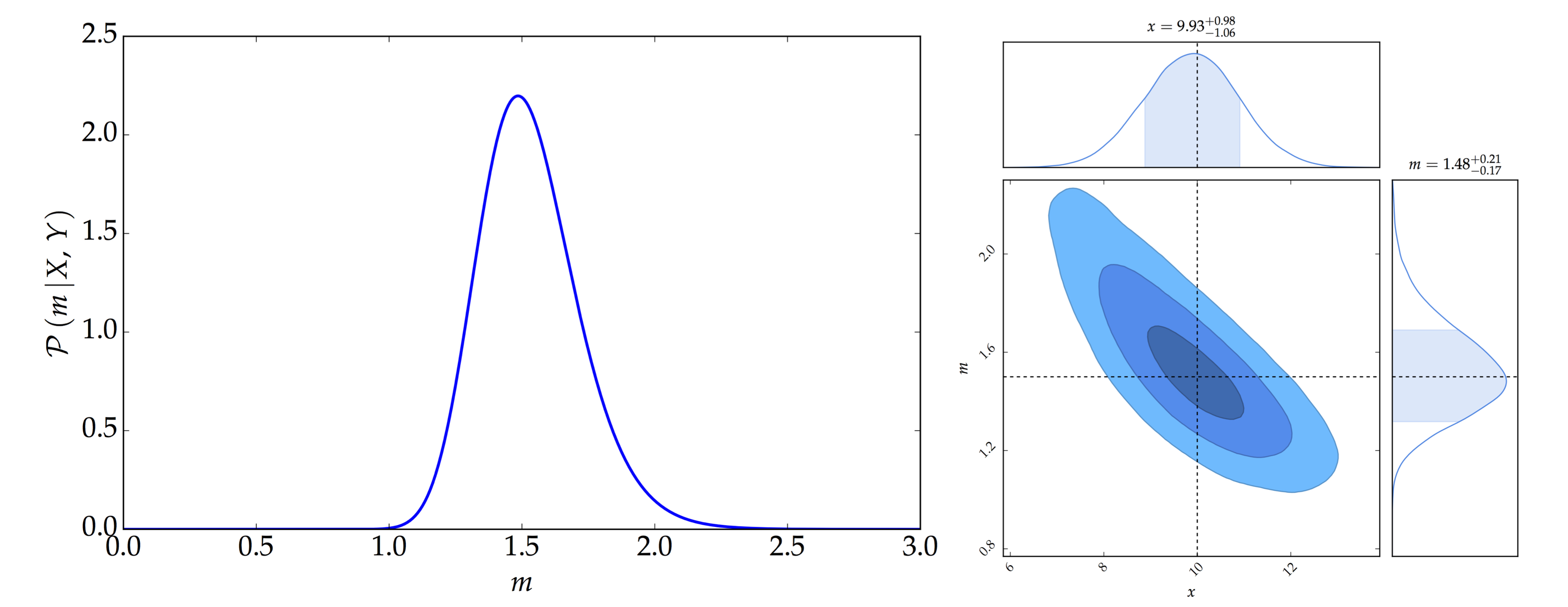
- The left panel shows the posterior distribution of $m$ while the right panel shows the joint posterior distribution of $x$ and $m$ using Gibbs Sampling.