Parameter Inference with MOPED and GP
In this post, I will cover briefly my first paper which was published in MNRAS during my PhD. An important step in this paper is the compression and emulation of the MOPED coefficients. MOPED is an algorithm developed by Heavens et al. 2000, which essentially compresses a data vector of size $N$ to just $p$ numbers, where $p$ is the number of parameters in the model. The first and subsequent MOPED vectors are given respectively by
\begin{align} \mathbf{b}_{1}=\frac{\mathbf{C}^{-1}\mathbf{\mu}_{,1}}{\sqrt{\mathbf{\mu}_{,1}^{\textrm{T}}\mathbf{C}^{-1}\mathbf{\mu}_{,1}}} \end{align}
and
\begin{align} \mathbf{b}_{\alpha}=\frac{\mathbf{C}^{-1}\mathbf{\mu}_{,\alpha}-\sum_{\beta=1}^{\alpha-1}(\mathbf{\mu}_{,\alpha}^{\textrm{T}}\mathbf{b}_{\beta})\mathbf{b}_{\beta}}{\sqrt{\mathbf{\mu}_{,\alpha}^{\textrm{T}}\mathbf{C}^{-1}\mathbf{\mu}_{,\alpha}-\sum_{\beta=1}^{\alpha-1}(\mathbf{\mu}_{,\alpha}^{\textrm{T}}\mathbf{b}_{\beta})^{2}}}\;\;(\alpha>1). \end{align}
The weighing vector, $\mathbf{b}$ encapsulates as much information as possible for a specific model parameter $\mathbf{\theta}_{\alpha}$. This vector is then used to find linear combination of the data, $\mathbf{d}$ such that the compressed data is
\begin{align} y_{\alpha}\equiv\mathbf{b}^{\textrm{T}}_{\alpha}\mathbf{d} \end{align}
and the expected theoretical prediction is simply $y_{\alpha}\equiv\mathbf{b}^{\textrm{T}}_{\alpha}\mathbf{\mu}$. One would then use an MCMC algorithm to sample the posterior distribution of the model parameters using the MOPED compression algorithm. In particular, each MOPED vector is orthogonal to each other and is also normalised, hence the log-likelihood is simply
\begin{align} \textrm{log}\,\mathcal{L} = -\frac{1}{2}\sum_{\alpha=1}^{p}(y_{\alpha}-\mathbf{b}_{\alpha}^{\textrm{T}}\mathbf{\mu})^{2} + \textrm{constant} \end{align}
However, calculating the MOPED coefficient at each step in an MCMC can be expensive if the forward model itself is expensive. Hence, a training set is first generated at $N$ Latin Hypercube samples (LHS) and the MOPED coefficients are computed at these points, followed by modelling $p$ separate Gaussian Processes. These are then used as surrogates to sample the posterior distribution of the model parameters and the result is shown in the figure below. The figure shows the posterior with the full accurate solver CLASS (in tan) and the posterior due to the emulator is shown in blue. The contours are plotted at 68% and 95% credible intervals.
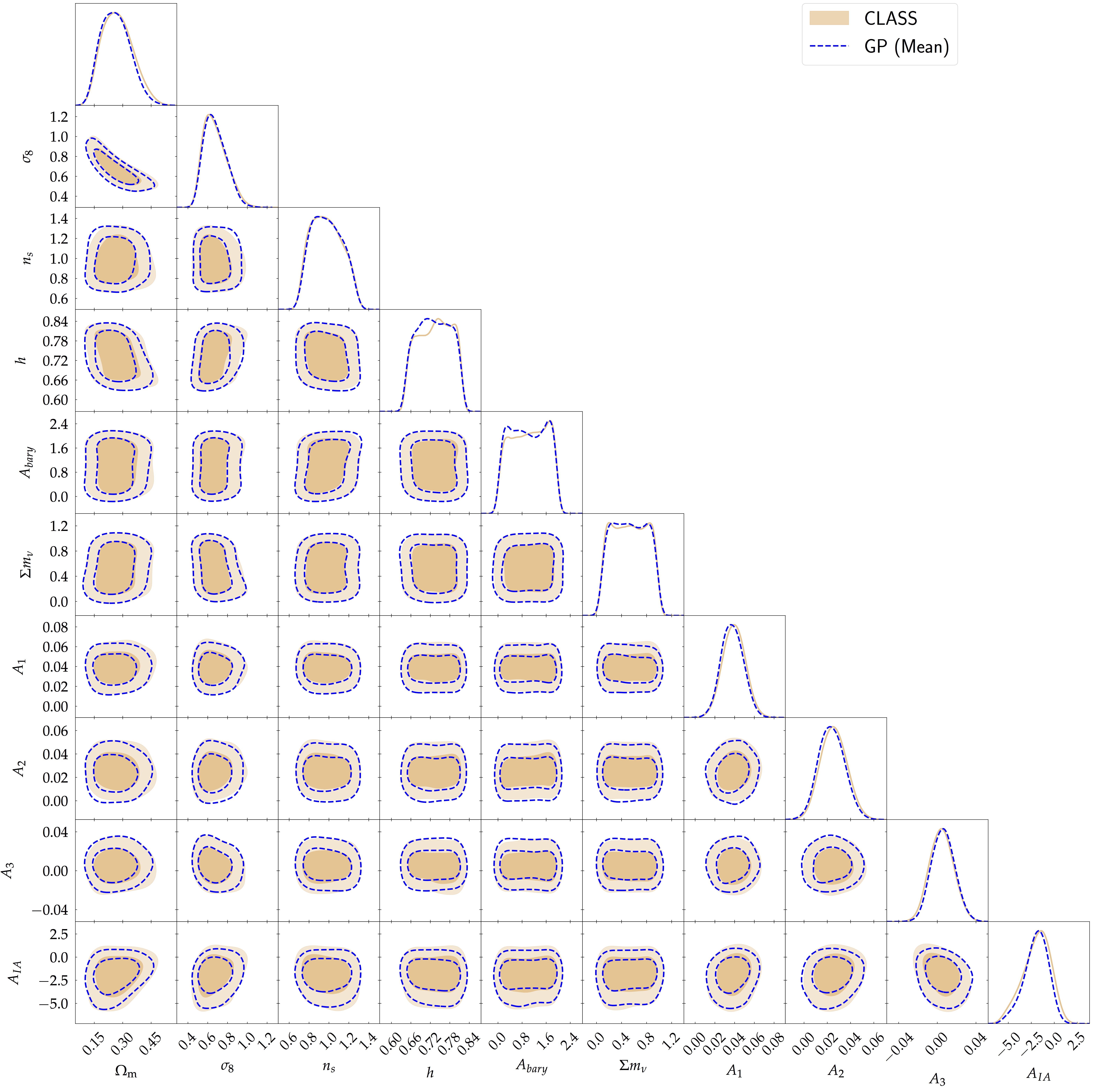
- The full posterior distribution of all parameters using the MOPED compression scheme.