Emulator for the 3D Matter Power Spectrum
The 3D matter power spectrum, $P_{\delta}(k,z)$ is a key quantity which underpins most cosmological data analysis, such as galaxy clustering, weak lensing, 21 cm cosmology and various others. Crucially, the calculation of other (derived) power spectra can be fast if $P_{\delta}(k,z)$ is precomputed. In practice, the latter is the most expensive component and can be calculated either using Boltzmann solvers such as CLASS or CAMB, or via simulations, which can be computationally expensive depending on the resolution of the experiments.
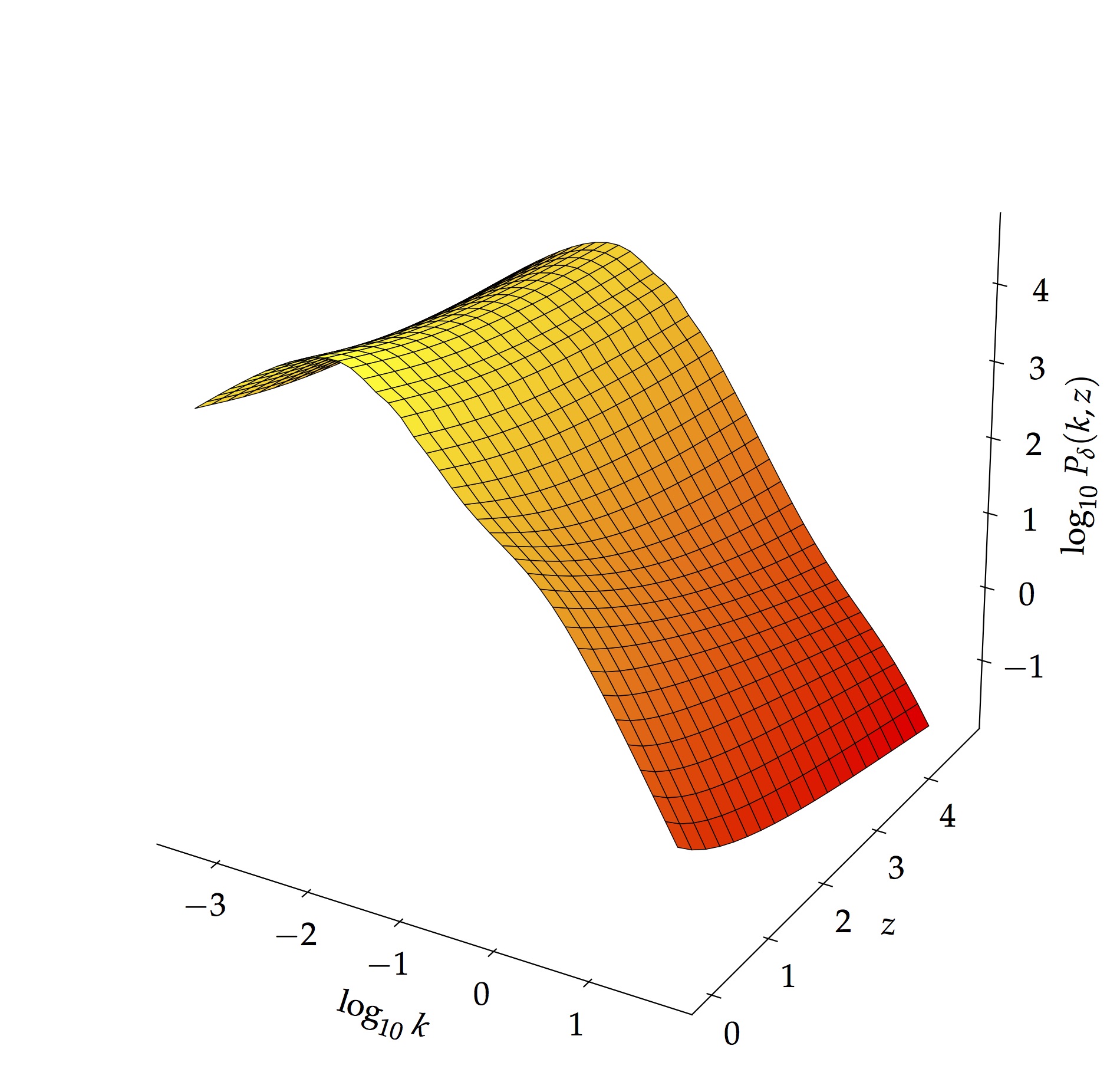
This work was published in the Astronomy and Computing journal. Our contributions in this work are three fold. First, it addresses the point that we do not always need to assume a zero mean Gaussian Process model for performing emulation, in other words, one can also include some additional basis functions prior to defining the kernel matrix. This can be useful if we already have an approximate model of our function. Moreover, if we know how a particular function behaves, one can adopt a stringent prior on the regression coefficients for the parametric model, hence allowing us to encode our degree of belief about that specific parametric model. Second, since we are using a Radial Basis Function (RBF) kernel and the fact that it is infinitely differentiable enables us to estimate the first and second derivatives of the 3D matter power spectrum. The derived expressions for the derivatives also indicate that there is only element-wise matrix multiplication and no matrix inverse to compute. This makes the gradient calculations very fast. Finally, with the approach that we adopt, we show that the emulator can output various key power spectra, namely, the linear matter power spectrum at a reference redshift $z_{0}$ and the non-linear 3D matter power spectrum with/without an analytic baryon feedback model. Moreover, using the emulated 3D power spectrum and the tomographic redshift distributions, we also show that the weak lensing power spectrum and the intrinsic alignment (II and GI) can be generated in a very fast way using existing numerical techniques. The 3D matter power spectrum can be decomposed as $$ P_{\delta}(k,z)=D(z)[1+q(k,z)]P_{\textrm{lin}}(k,z_{0}) $$ Each component $D(z)$, $q(k,z)$ and $P_{\textrm{lin}}(k,z_{0})$ are then modelled as separate semi-parametric Gaussian Processes, where we assume a second order polynomial function for the parametric part.
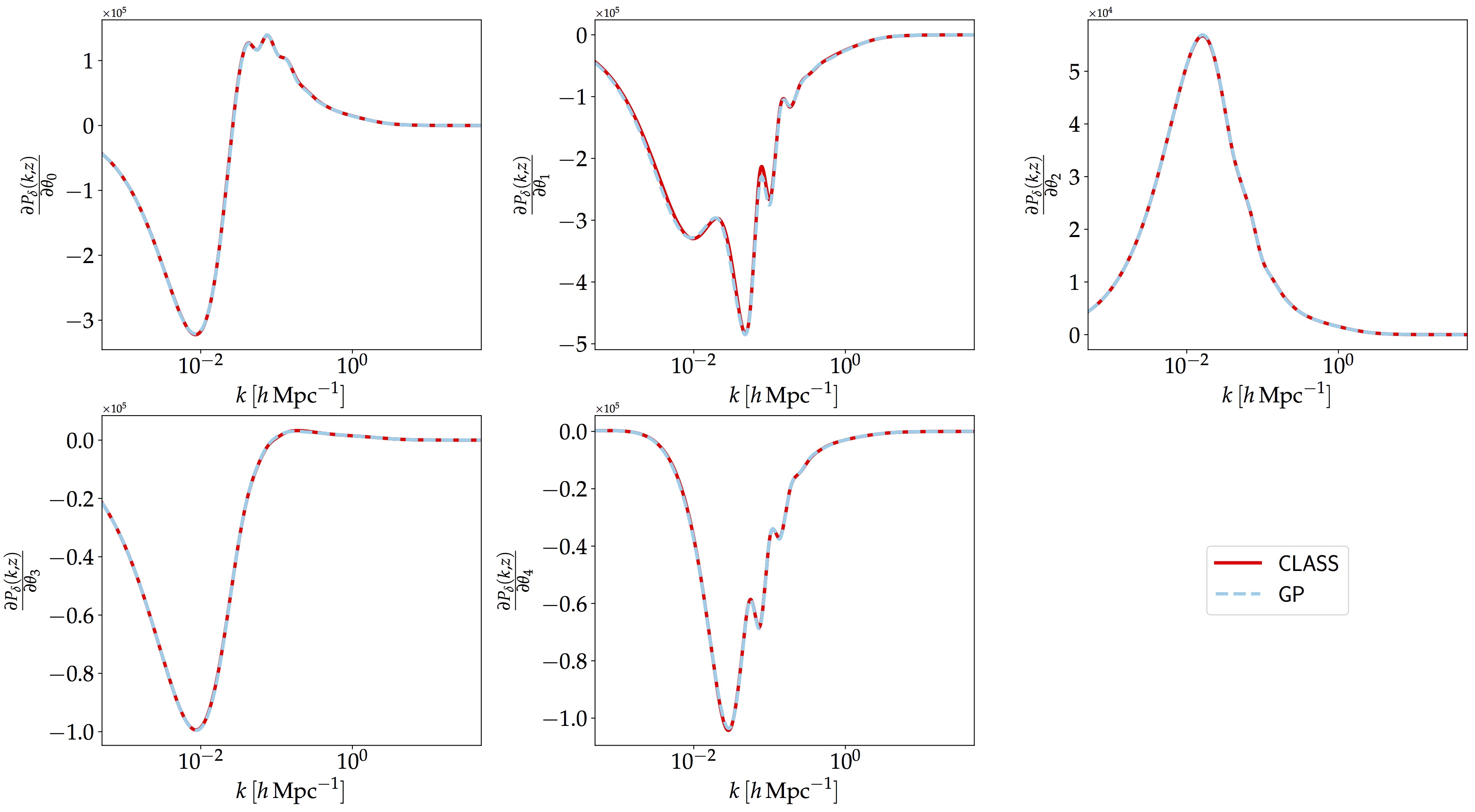
- The gradients of the power spectrum with respect to each cosmological parameter at a fixed redshift.
In the figure above, we show the gradient along at a fixed cosmological parameter (test point) and fixed redshift, $z=0$. The red curve corresponds to the gradients as calculated by CLASS using central difference method and the blue curves show the gradients output from the emulator. In particular, this gradient is strictly a 3D quantity, as a function of the wavenumber $k$, redshift, $z$ and the cosmological parameters $\boldsymbol{\theta}$. In other words, the gradient calculation from the emulator will be a tensor of size $(N_{k},\,N_{z},\,N_{p})$, where $N_{k}$ is the number of wavenumbers for $k\in[5\times 10^{-4},\,50]$, $N_{z}$ is the number of redshifts for $z\in[0.0,\,5]$ and $N_{p}$ is the number of parameters considered. In this case, $N_{p}=5$ and the default values for a finer grid in $k$ and $z$ are $N_{k}=1000$ and $N_{z}=100$ respectively.
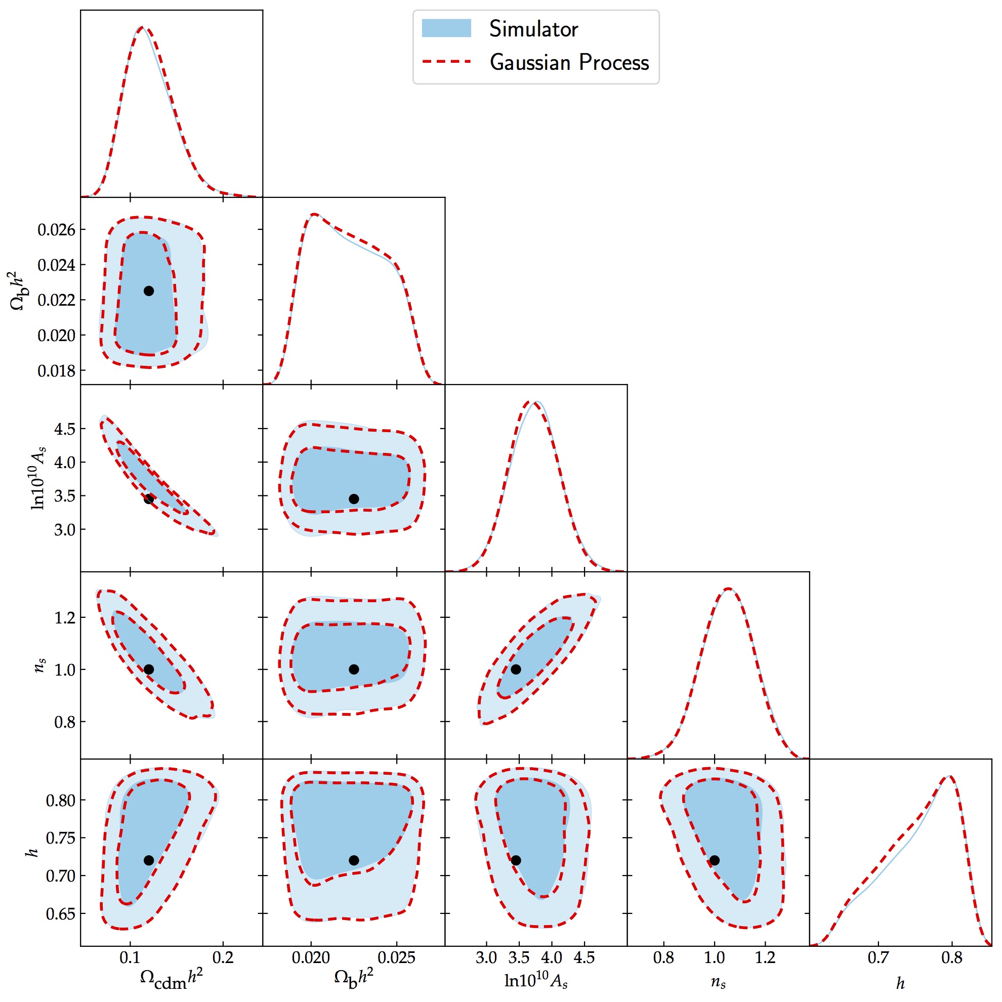
- The full posterior distribution of all parameters using the emulator on a toy dataset.
We also test the emulator on simulated weak-lensing bandpowers. We assume measurements over $10\leq\ell\leq 1500$ and 5 tomographic slices with Gaussian $n(z)$ centred on redshifts [0.5, 1.0, 1.5, 2.0, 2.5] and each having a standard deviation of 0.075. Ten bandpowers, equally spaced in logarithmic scale, are used and this gives us a set of 150 data points. Moreover, we simulate and then assume in the likelihood independent Gaussian errors with, for simplicity, $\sigma=0.5\hat{\mathcal{B}}_{\ell}$, where $\hat{\mathcal{B}}_{\ell}$ is the bandpower evaluated at the fiducial set of cosmological parameters. For this particular case, we have set $A_{\textrm{IA}}=0$ but one can trivially include this factor and marginalise over it in the sampling process. The fiducial point $\boldsymbol{\theta}_{\textrm{fid}}=[0.12, 0.0225, 3.45, 1.0, 0.72]$ is used to generate the data and is shown by the black dots in the figure above. We use a Gaussian likelihood and uniform priors on all cosmological parameters, similar to the range of the inputs of the emulator. The figure below shows the results obtained when sampling the cosmological parameters on this toy data set. The red contours correspond to the result using the emulator while the pale blue colour refers to the posterior distributions using CLASS. We run three separate MCMC chains, each with 150 000 MCMC samples, two with the emulator and one with CLASS. On each of the three resulting pairs of runs, we compute the Gelman-Rubin convergence parameter. The worst $\hat{R}$ value is 1.002, consistent with all three chains being drawn from the same distribution, and corroborating the agreement shown in the above figure. The emulator developed in this work is thus able to robustly recover the posterior distributions of all the cosmological parameters, compared to the accurate solver, CLASS.