emuflow: Combining Experiments with Normalising Flows

In this post, I briefly summarise emuflow, written at Oxford with Carlos García-García, David Alonso and Jaime Ruiz-Zapatero. The question is simple: if several experiments have already published MCMC chains, can we combine them without re-running their expensive likelihoods?

The problem

Each experiment constrains a small set of shared cosmological parameters $\boldsymbol{\theta}$, but also carries its own nuisance parameters $\boldsymbol{\beta}_i$ (galaxy biases, calibration, redshift shifts and so on). With $b$ cosmological parameters and $c_i$ nuisance parameters per experiment, a joint analysis samples $b+\sum_i c_i$ dimensions, and every step calls every experiment's forward model. The dimension and the cost both grow with each dataset added.

Yet most of the time, we only care about $p(\boldsymbol{\theta}\,|\,\boldsymbol{x}_i)$, the posterior with the nuisance parameters marginalised out. Existing chains already contain samples from it: we just drop the nuisance columns. What is missing is a density we can evaluate.

The idea

A normalising flow starts from a simple distribution, such as a Gaussian, and passes it through a sequence of invertible neural network transformations that stretch and bend it into the shape of the target posterior. Because every step is invertible, the flow can both generate new samples and evaluate the density at any point, which is exactly what we need. Training is maximum likelihood on the chain samples. We use an affine autoregressive flow, which keeps the density calculation cheap. About 20,000 samples train a flow over five or six parameters in roughly two minutes on a desktop.

Once each experiment has a flow, there are two ways to use it. A legacy experiment's flow can act as an informative prior for the likelihood of a new one, so the old nuisance parameters and forward model disappear from the analysis. Alternatively, the flows alone can be multiplied together (a product of experts), correcting for the shared prior:

\[p(\boldsymbol{\theta}\,|\,\boldsymbol{x}_1,\ldots,\boldsymbol{x}_N) \propto p(\boldsymbol{\theta}) \prod_{i=1}^{N} \frac{p_{\textrm{nf}}(\boldsymbol{\theta}\,|\,\boldsymbol{x}_i)}{p(\boldsymbol{\theta})}.\]

A hard test

We validated the method on a deliberately difficult pair: Planck 2018 and a large combination of large-scale structure data (galaxy clustering, weak lensing and CMB lensing), which disagree on $S_8$ at about $3.5\sigma$. Their joint posterior sits in the tails of each individual one, so a flow that only captures the bulk would fail.

• Planck flow as a prior: posterior means are recovered at the sub-percent level and widths within 2–3%. The exact joint run took about 24 days on two HPC nodes; this took about 6.
• Two flows only: the joint posterior takes under 15 minutes on a desktop. The price is accuracy: means shift by up to about $0.3\sigma$, which is expected given how much the result relies on the tails.

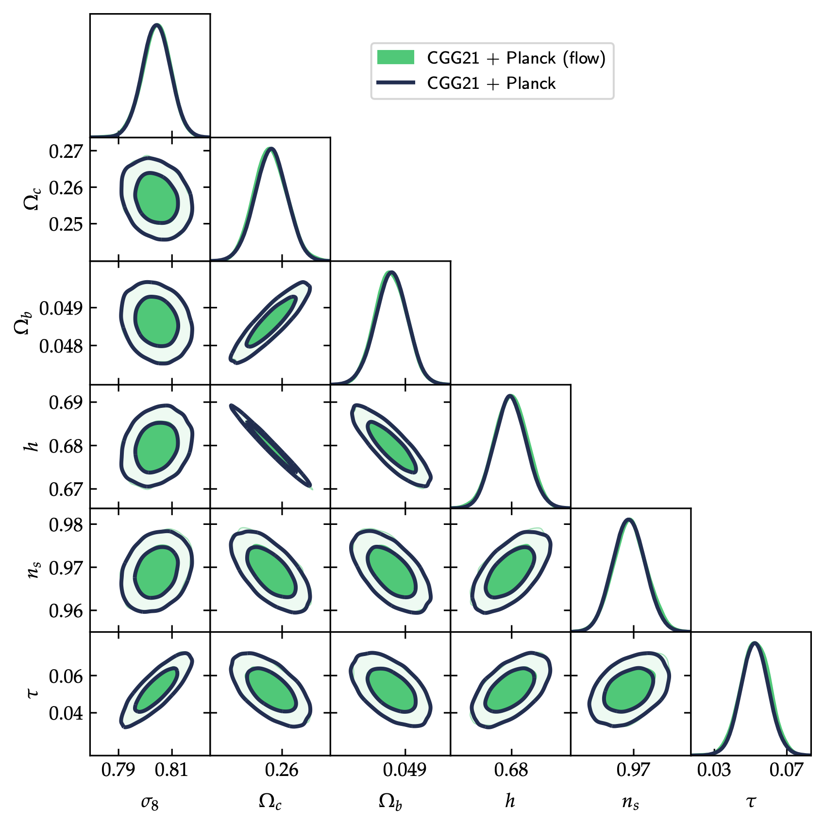
Further tests, combining KiDS-1000 with DES Y3 and Planck with DES Y1, involve milder tension but less Gaussian posteriors, and lead to the same conclusions.

A zoo of pre-trained flows

We also trained flows on public chains from Planck 2018, DES Y3, KiDS-1000, ACT DR4 and SDSS, and released them with the code. Adding a new experiment or extending the cosmological model only needs its MCMC samples and a few minutes of training.

One caveat: the combination rule assumes independent datasets and uninformative priors on $\boldsymbol{\theta}$ in each original analysis. A chain that already includes another experiment as a prior would count that information twice.