Bayesian Evidence - The Gaussian Linear Model

Following our recent post on Bayesian Model Selection, here we will illustrate it using a simple example of the Bayesian Evidence calculation using the Gaussian Linear Model. Consider the figure below.

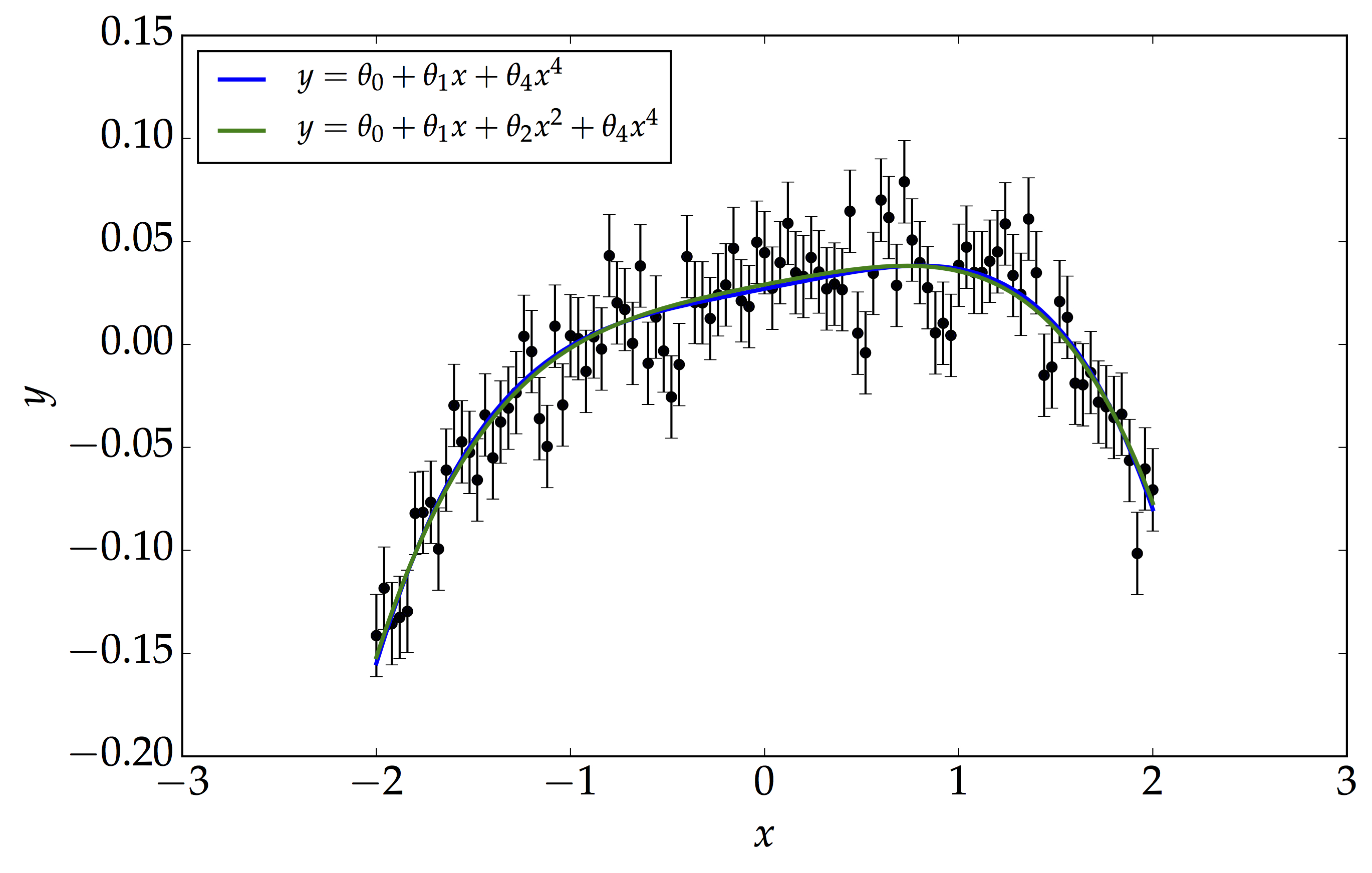
We have our data, which is dominated by noise, $\mathbf{n}\sim\mathcal{N}\left(0,\,0.02\right)$. Here, we are motivated to consider two models, $\mathcal{M}_{1}$ and $\mathcal{M}_{2}$, given by $$ y=\theta_{0}+\theta_{1}x+\theta_{2}x^{2}+\theta_{4}x^{4} $$ $$ y=\theta_{0}+\theta_{1}x+\theta_{4}x^{4} $$ It is actually very hard to choose the best model just by looking at the fit. Note that the fitting method used here is the Maximum a Posteriori method, MAP where we assume the prior on each parameter is Gaussian distributed with mean 0 and variance 1, that is, $\theta_{i}\sim\mathcal{N}\left(0,\,1\right)$. Moreover, setting $\theta_{2}$ to zero reduces $\mathcal{M}_{1}$ to $\mathcal{M}_{2}$. This is a common scenario in various fitting problem we deal with in Statistics. If we naively perform a $\chi^{2}-$test, then the model with the larger number of parameters will always be selected. This is a case of overfitting we encounter and we should be cautious about it. The notation we will be using are: $\mathbf{D}$ as the design matrix and $\mathbf{P}$ as the covariance matrix for the priors. See here for further details on $\mathbf{D}$ and $\mathbf{b}$. The Bayesian Evidence is given by $$ \mathbb{Z}=\mathcal{P}\left(\mathcal{D}\left|\mathcal{M}\right.\right)=\int\mathcal{P}\left(\mathcal{D}\left|\boldsymbol{\theta},\,\mathcal{M}\right.\right)\mathcal{P}\left(\boldsymbol{\theta}\left|\mathcal{M}\right.\right)d\boldsymbol{\theta} $$ $$ \mathbb{Z}=\left(\sqrt{\left|2\pi\mathbf{P}^{-1}\right|}\,{\prod_{i}}\sqrt{2\pi\sigma_{i}^{2}}\right)^{-1}\int\textrm{exp}\left[-\dfrac{1}{2}\left\{ \left(\mathbf{b}-\mathbf{D}\boldsymbol{\theta}\right)^{\textrm{T}}\left(\mathbf{b}-\mathbf{D}\boldsymbol{\theta}\right)+\mathbf{\boldsymbol{\theta}}^{\textrm{T}}\mathbf{P}^{-1}\mathbf{\boldsymbol{\theta}}\right\} \right]\,d\boldsymbol{\theta} $$

Using the above two important tricks, the Bayesian Evidence is:

where $\mathbf{k}=-\left(\mathbf{D}^{\textrm{T}}\mathbf{b}\right)^{\textrm{T}}\left(\mathbf{D}^{\textrm{T}}\mathbf{D}+\mathbf{P}^{-1}\right)^{-1}\left(\mathbf{D}^{\textrm{T}}\mathbf{b}\right) $ Using the above results, the log-Bayesian Evidence for the two models, $\mathcal{M}_{1}$ and $\mathcal{M}_{2}$ are 238.458 and 243.338 respectively. Therefore, the log-Bayes Factor, $\textrm{log B}_{21}$, which is simply the difference between the two numbers is 4.88, thus showing that $\mathcal{M}_{2}$ is strongly favoured model over $\mathcal{M}_{1}$ (refer to the Jeffreys’ scale in our previous blog post).

SDDR - Savage-Dickey Density Ratio

Savage-Dickey Density Ratio (SDDR) is a useful method for comparing nested models and is in fact, a good approximation to the Bayes Factor. For some parameter values, the extended model $\mathcal{M}_{1}$ reduces to the simpler model $\mathcal{M}_{0}$. Consider a complex model made up of two sets of parameters $\boldsymbol{\theta}=\left(\boldsymbol{\psi},\,\boldsymbol{\phi}\right)$ and the simple model is obtained by setting $\boldsymbol{\phi}=\boldsymbol{\phi}_{0}$. If we further assume that the priors are separable, which is a common scenario: $$ \mathcal{P}\left(\boldsymbol{\psi},\,\boldsymbol{\phi}\left|\mathcal{M}_{1}\right.\right)=\mathcal{P}\left(\boldsymbol{\psi}\left|\mathcal{M}_{1}\right.\right)\mathcal{P}\left(\boldsymbol{\phi}\left|\mathcal{M}_{1}\right.\right) $$ then, the Bayes Factor can, in principle, be written as \begin{equation} B_{01}=\left.\dfrac{\mathcal{P}\left(\boldsymbol{\phi}\left|\mathcal{D},\,\mathcal{M}_{1}\right.\right)}{\mathcal{P}\left(\boldsymbol{\phi}\left|\mathcal{M}_{1}\right.\right)}\right|_{\boldsymbol{\phi}=\boldsymbol{\phi}_{0}} \end{equation} The above equation is referred to as the Savage-Dickey Density Ratio. In short, the SDDR is simply the ratio of the marginal posterior to the prior of the complex model, evaluated at the nested point, that is, at the simpler model's parameters value. The SDDR is important to judge whether the inclusion of extra parameters in nested models are important when we are trying to fit the observed data. Moreover, in most problems, it is computationally challenging to compute the Bayesian Evidence and hence the Bayes Factor, as it is a multi-dimensional integral. The SDDR provides an alternative avenue to compute the Bayes Factor without computing the Bayesian Evidence provided the models are nested.