Iterative Method For Likelihood Emulation
The paper, entitled 'Cosmological parameter estimation via iterative emulation of likelihoods' was published on arXiv recently. The idea behind is to use Gaussian Process to emulate the log-likelihood and to progressively augment the training set via Bayesian Optimisation. In this post, I shall illustrate the technique via simple straight line fitting example, which I believe will be trivial to follow.
Analytical Posterior
To start with, we randomly draw 50 points uniformly from $x\in[0, 1]$ and compute $\mathbf{y}$, which is given by $$ \mathbf{y} = \theta\mathbf{x} + \boldsymbol{\epsilon} $$
We fix $\theta = 1$ and $\boldsymbol{\epsilon}\sim\mathcal{N}(0, 0.04^{2})$. We also assume a Gaussian prior for $\theta$, where $p(\theta)=\mathcal{N}(1,1)$. The posterior distribution of $\theta$ can be derived analytically and is in fact another Gaussian distribution, given by: $$ p(\theta|\mathbf{y}) = \mathcal{N}(\mu, \sigma^{2}) $$ where
- $\mu = 625\sigma^{2}\mathbf{D}^{\textrm{T}}\mathbf{y}$
- $\sigma^{2}=(1 + 625\mathbf{D}^{\textrm{T}}\mathbf{D})^{-1}$
- $\mathbf{D} = [x_{0},\,x_{1},\ldots x_{N-1}]^{\textrm{T}}$
with the factor 625 arising due to 1/0.042.
Gaussian Process and Bayesian Optimization
Gaussian Process is a joint multivariate Gaussian distribution over functions with a continuous domain. We will not cover it in this post (for further details, see here). The predictive distribution is a Normal distribution with mean and variance given respectively by: $$ f_{*} = \mathbf{k}_{*}^{\textrm{T}}\mathbf{K}^{-1}\mathbf{y}_{\textrm{train}} $$ $$ \sigma_{*}^{2} = k_{**} - \mathbf{k}_{*}^{\textrm{T}}\mathbf{K}^{-1}\mathbf{k}_{*} $$ On the other hand, Bayesian Optimization is a proxy for finding the optima of expensive objective functions via the acquisition function, which we will discuss briefly below. A typical example of expensive computation is in cosmology where we have a series of multiple integrations and other expensive computations (for example, when we also have to account for the systematics) prior to computing the log-likelihood in a Bayesian analysis.
Acquisition Functions
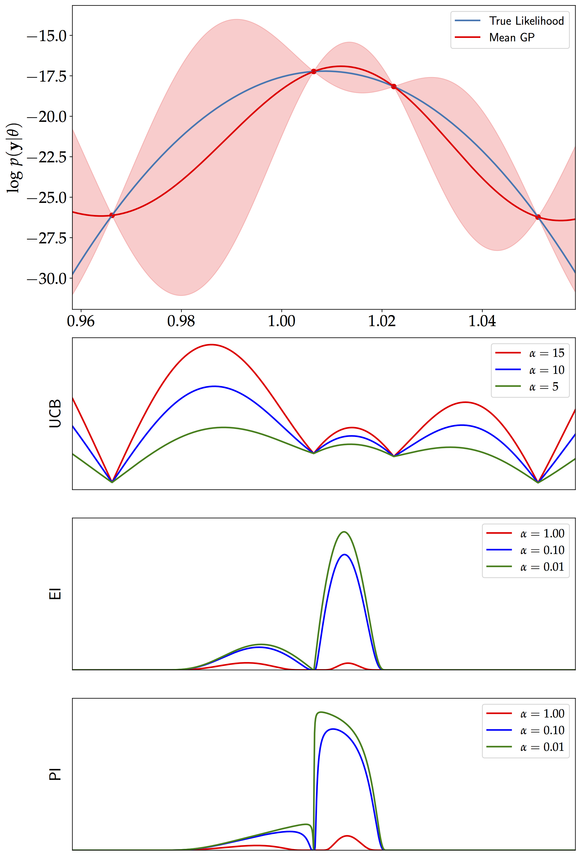
One class of acquisition function (also referred to infill function) is improvement-based function. Probability of improvement (also called maximum probability of improvement or the P-algorithm) is one such example and is given by: $$ \textrm{PI}(\theta) = \Phi(z) $$ In the same spirit, the expected improvement does not only consider the probability of improvement but also takes into account the magnitude of improvement that the additional point will provide. It reads: $$ \textrm{EI}(\theta)=\begin{cases} \begin{array}{c} \left(\mu-f_{\textrm{max}}-\alpha\right)\Phi(z)+\sigma\phi(z)\\ 0 \end{array} & \begin{array}{c} \textrm{if }\sigma>0\\ \textrm{if }\sigma=0 \end{array}\end{cases} $$ where $\Phi(\centerdot)$ and $\phi(\centerdot)$ correspond to the Cumulative Distribution Function (CDF) and Probability Distribution Function (PDF) of a normal distribution respectively. $f_\textrm{max}$ refers to the maximum of the expensive function, given a set of inputs, $\theta$ and $$ z(\theta) = \frac{\mu(\theta) - f_{\textrm{max}} - \alpha}{\sigma(\theta)}. $$ On the other hand, another acquisition function based on upper confidence bound is given by: $$ \textrm{UCB}(\theta) = \mu + \alpha \sigma $$ Note the additional parameter $\alpha$ in the acquisition functions. It is usually user-defined and it essentially controls the trade-off between exploration (region of high uncertainty) and exploitation (region with high mean).Our Implementation
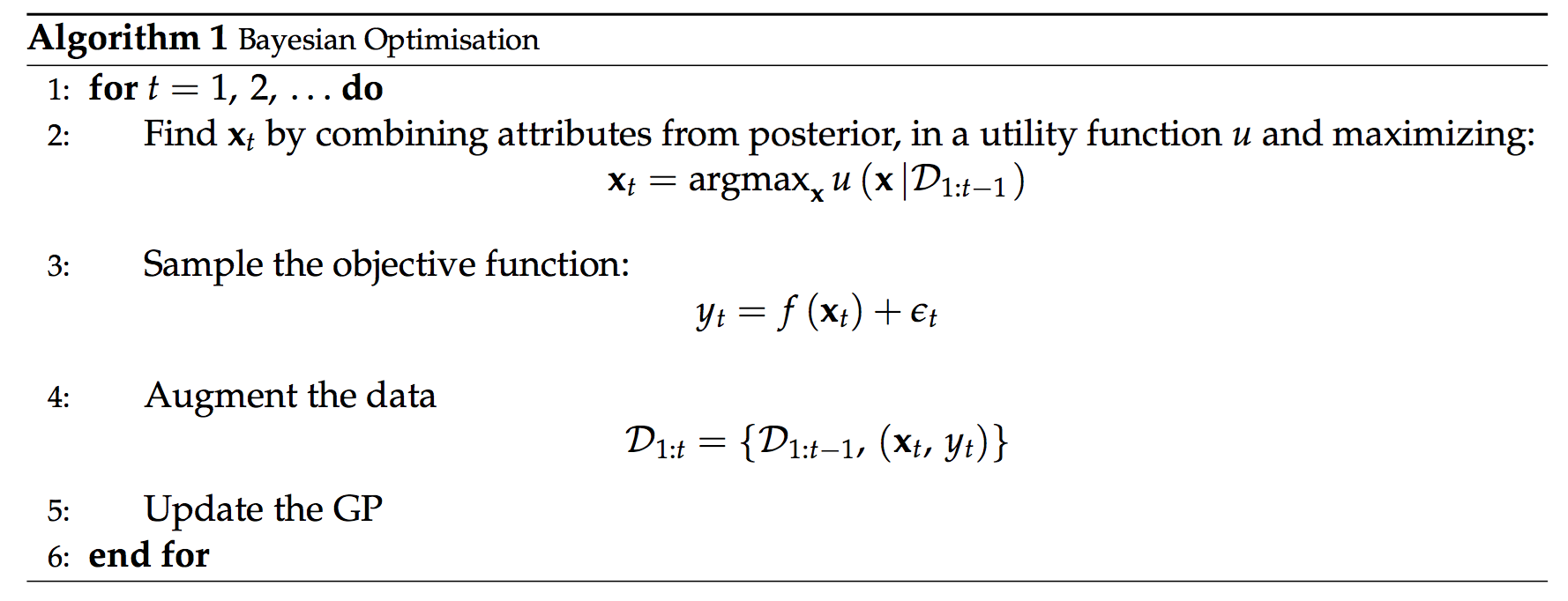
We initially start with just 4 training points (generated using Latin Hypercube samples, LHS) given by the first 4 rows in the table at the bottom. We then use the Upper Confidence Bound (UCB) acquisition function (with $\alpha=15$) to iteratively add two points (the last two rows in red in the table) to the Gaussian Process model. See algorithm below for further details.
| $\theta$ | $\textrm{log } L$ |
|---|---|
| 0.9662 | -26.1204 |
| 1.0064 | -17.2318 |
| 1.0223 | -18.1605 |
| 1.0511 | -26.2248 |
| 0.9860 | -19.7343 |
| 1.0369 | -21.2069 |
Results and Conclusions
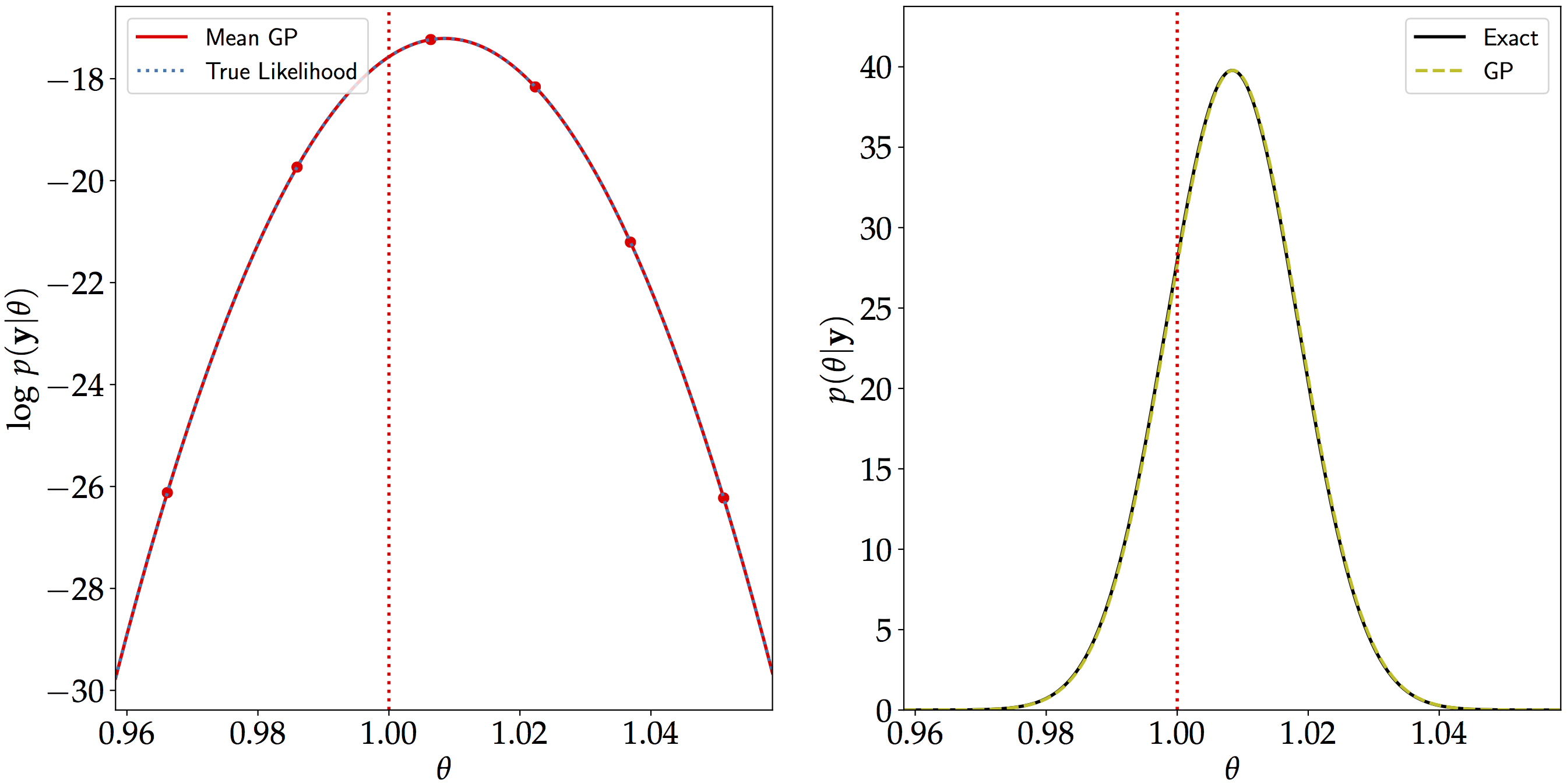
In this setup, we are able to reconstruct the log-likelihood almost perfectly after augmenting the data set in two iterations. As seen in the plot below in the right panel, the posterior distribution of $\theta$ is identical to the exact one (which we calculated analytically previously). The vertical broken line shows the value of $\theta=1$ which we initially used to generate the data.
However, in high dimensions, the volume of the parameter space increases and it is not easy to reconstruct a function perfectly (if this is the main objective). Moreover, the acquisition functions themselves contain multiple local optima (as seen in the Figure on the top) and the choice of the acquisition function is an interesting topic. They can often be greedy and favour exploitation over exploration, hence the choice of $\alpha$ also matters.
References